SICP Chapter 1.2, notes and (some) solutions in Clojure

Summary: Review of some parts of Chapter 1.2 of SICP: execution of processes, recursion versus iteration, growth. A few selected exercises.

The previous chapter introduced the elements of programming, the basic building blocks to express ideas by defining procedures. Chapter 1.2 goes one step further by examining what happens if a procedure gets executed. Predicting how a process is going to behave is not an easy task, but as a first step we introduce some typical execution patterns.

Iteration versus recursion

Depending on how a procedure is defined, the generated process can have very different behaviour. One fundamental distinction can be made between iterative and recursive processes.

A recursive process “expands” in memory by building up a chain of deferred evaluations. This kind of process has two phases: first building up the chain by continuously applying the substitution model, until no substitutions are left to be done (“expansion”), and then, in a second phase (“contraction”), applying the operations until the final result is calculated.

(The fact that a recursion expands might be the reason why grasping it can be difficult sometimes).

An iterative process on the other hand, does not “expand”. To calculate the end result, the procedure introduces a parameter (a state) that keeps track of the intermediate results until the calculation is done. An iterative process, therefore, can be stopped anytime and the calculation can be re-started from where it has been left off. That would not be possible with a recursive process, as the expanded state would get lost between restarts.

Recursive procedure != recursive process

One important conclusion is that a recursive procedure does not necessarily generate a recursive process. We can define a recursive procedure (by referencing to itself), but the resulting procedure can still be iterative.

Growth

The first examples in the chapter (e.g. calculation of n!) are processes that grow linear with the size of the argument (e.g. the size of n). Growth is usually measured in space and steps. Space that is required to store each calculation step and steps that are needed until the calculation finishes. The order of growth can be any form like constant, linear, exponential and so on. Another execution pattern is processes that generate a tree recursion. Here, steps equal the number of nodes and space the maximum depth of the tree (the whole branch in the recursion tree needs to be kept in memory for the calculation of the leave).

This chapter deals mostly with growth.

Exercises

Source code and some more solutions can be found in my Github repo¹.

1.9 Evaluation of iteration and recursion

Given two procedures that define addition, which one creates a recursive process and which an iterative?

The first procedure:

(defn + [a b]
  (if (= a 0) b
      (inc (+ (dec a) b))))

If we apply the substitution model, we get following steps:

(+ 4 5)
(inc (+ 3 5)
(inc (inc (+ 2 5))
(inc (inc (inc (+ 1 5)))
(inc (inc (inc (inc (+ 0 5))))
(inc (inc (inc (inc 5)))
(inc (inc (inc 6))
(inc (inc 7))
(inc 8)
9

As we can easily see, this is a recursive process that expands and contracts.

The second procedure:

(defn + [a b]
  (if (= a 0) b
    (+ (dec a) (inc b))))

The process looks like this:

(++ 4 5)
(++ 3 6)
(++ 2 7)
(++ 1 8)
(++ 0 9)
9

An iterative process that keeps a state and does not expand.

Is there a way to “see” whether a process is recursive or not? The key to answering this question is the fact that recursion defers evaluation. This is what happens in the procedure body: (inc (+ (dec a) b)) defers the evaluation of inc until (+ (dec a) b) terminates. In the second example, this is not the case: (+ (dec a) (inc b)) does not defer the evaluation of +, because the arguments (dec a) and (inc b) can be immediately evaluated.

1.11 Finding an iterative solution

Another exercise about recursion versus iteration: write procedures of the following function that result in an iterative and recursive process:

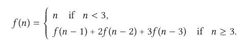
The recursive solution can be translated straight from the mathematical definition:

(defn f [n]
  (if (< n 3) n
    (+ (f (- n 1)) (* 2 (f (- n 2))) (* 3 (f (- n 3))))))

This is an example that shows how recursion is often a much more straight-forward way of defining procedures. To see that this generates a recursive process, we can look at one the of the operands, e.g. (* 3 (f (- n 3))): here, the * operation is deferred until (f(- n 3)) terminates.

To come up with an iterative solution, we need to do a bit of thinking beforehand. To start, lets write down a few of the first iterations:

f(0)  = 0
f(1)  = 1
f(2)  = 2
f(3)  = f(2) + 2 * f(1) + 3 * f(0)
      =   2  + 2 *  1   + 3 *  0
      = 4
f(4)  = f(3) + 2 * f(2) + 3 * f(1)
      =  4   + 2 *   2  + 3 * 1
      = 11

For n >= 3, if we write the three summands as:

  = a + b + c

we notice that in each iteration following substitions happen:

a = f(a)
b = 2 * a
c = 3 * b

so all we have to do is start the iteration with the correct values for n = 3 (a = 2, b = 1, c = 0), and iterate until n < 3 and the result is stored in a

(defn f-iter [a b c step]
  (if (< step 3) a
      (f-iter (+ a (* 2 b) (* 3 c)) a b (- step 1))))

(defn fi [n]
  (if (< n 3) n
      (f-iter 2 1 0 n)))

In this procedure, no operation gets deferred, and the combination of the procedure parameters a b c step introduce a state that stores the intermediate results of each iteration.

Exercise 1.14 Tree recursion

In this exercise, we are supposed to draw the evaluation tree of the count change procedure that was defined in the text and determine the order of growth of space and steps. It’s mostly an exercise to get a feel for how recursion expands into a tree. While doing this, the key points to remember are the termination rules:

• if amount is 0 then we count this as 1 way to make a change (think as if the change matches the amount, so we have found a valid way to make a change).
• if n (available coins to make a change) is 0 or if amount is negative we count this as 0 ways to make a change (think of negative amount that we have already “overshoot” the ways to make a change, and if no available coins are left we can’t make a change either).
• all other cases need further processing.

I have made a drawing of the evaluation tree. The grey nodes are 0, and the blue notes are 1

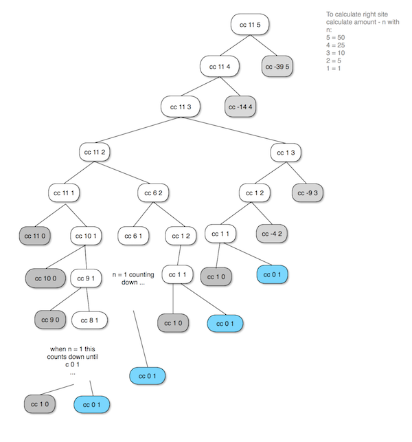
Counting the “blue” nodes, the result is 4.

I simplified the drawing. Observing that once a node reaches the state cc amount 1, the process is going to count down until it reaches cc 0 1 which counts as 1.

This gives us the answer to what growth of space is required by the process. The space is equal to the maximum depth of the tree. As the tree always counts down once n becomes one, the required space equals O(n+5) = O(n), so space grows linear.

The steps required by the process equals the number of nodes in the tree. The solution is not as obvious as it is for the space. As a very broad approximation, lets consider a generic tree that starts with cc n 5. The left side of each node converges to cc n 1 which has O(n) complexity. The right site starts with cc n-d 5, then cc n-2*d 5 and so on. In general, cc n-k 5, each node generating another subtree. This happens also for cc n 4, cc n 3, cc n 2, cc n 1. So using a very rough simplification, each subtree grows by multiplying O(n*n), and as there are 5 denominations the complexity is approximately O(n^5)